BIOL4585

Association Testing

Overview

Last week, you used gatk and samtools to map sequencing data to a reference genome, and generate a .vcf file. While your work involved a single chromosome for a single individual, GWAS often use thousands of times more data! In this week’s set of activities, you will perform a subsequent step of GWAS: the actual association part. You will be using plink, a commonly-used tool that measures statistic signals of association. Using it will require simulated data for 500 individuals, including two inputs:

Genotype data (from a .vcf file)
Phenotype data (in a special file format)

What are the statistics of genetic association testing in GWAS?

At the most basic case, associations are measured by a Chi-square test for differences in allele counts in two groups:

the case group, or those affected by a disease or condition
the control group, or those not affected by a disease or condition

Imagine 100 case individuals and 100 control individuals are genotyped at a candidate SNP implicated in a disease. Because humans are diploid, that means there will be a total of 200 alleles (two per individual) per group. Say the data falls out like so, with individuals having either a G or a C allele:

	case	control	total
G	125	97	222
C	75	103	178
total	200	200	400

These values are then used in a Chi-square test. You can run it here.

What is the chi-square statistic and p-value for the above table? Would you consider this considered a statistically significant result? Why?

Expected output from a GWAS

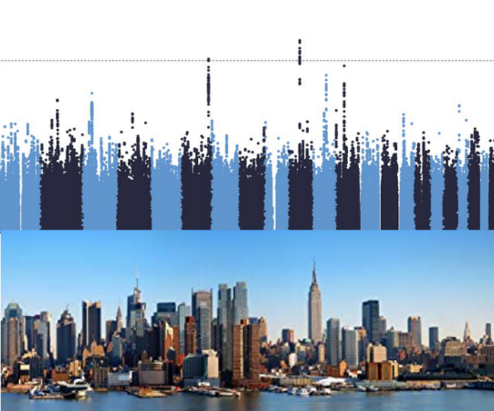
When running a GWAS, you are essentially running thousands and thousands of Chi-square tests–one for every locus (row) in a VCF file. In the end, you have a collection of genome positions (plotted on the X-axis) and significance scores (on the Y-axis). This form of displaying results is called a Manhattan plot. The name comes from the idea that when there are lots of SNPs, it looks like a city skyline, like that of Manhattan.

I’ve provided a VCF file MT.500.vcf that contains simulated genotype data for 500 individuals. You need to incorporate their phenotypic data together with genotype data to determine if any SNPs are associated with a modeled disease.

Examine the contents of MT.500.vcf. I recommend using less -S to disable word-wrap, making the file simpler to examine.

The format of a phentotype file

For this exercise, you have access to phenotype data in two separate files: a list of control individuals is within healthy.txt and a list of case individuals is within diseased.txt.

Your task is to generate a .pheno file by processing healthy.txt and diseased.txt using bash commands. The first two columns will both be the same value, followed by the phenotype in the third column. In this file format, a phenotype value of 1 means healthy, and a phenotype of 2 means diseased. You can use loops, awk, or sed plus the tools you already know. Save your commands to a text file for safekeeping. You will want it for later. See instructions here on formatting files using bash loops, awk, and sed.

The result will ultimately be a file organized like so:

FID	SID	PHENO
sample1	sample1	1
sample3	sample3	1
sample4	sample4	1
sample6	sample6	1
sample2	sample2	2
sample5	sample5	2
sample7	sample7	2
sample8	sample8	2

…etc.

Note: The above headers can be included in the .pheno file, but are not required. The sample and phenotype values above are just examples–your file will likely look different

Running an association test in Plink

Once you believe your .pheno file is properly formatted, execute a case-control analysis using plink.

Get Plink. Download it from its hosting website and extract the .zip archive. The file is hosted at https://www.cog-genomics.org/plink2/ and you want the stable build for Linux (64-bit).
Run a case-control association test. You will need to run the --assoc model, the --vcf option followed by an input .vcf filename, the --pheno option followed by your input .pheno filename. You can specify the output with --out prefix which will give you output files prefix.assoc, prefix.log etc. Note: you may need to specify an additional option. plink will complain to you if this is the case.

prefix.assoc is the output of the association test. Look through its contents, which includes the fields

column	meaning
CHR	Chromosome
SNP	SNP ID
BP	Physical position (base-pair)
A1	Minor allele name (based on whole sample)
F_A	Frequency of this allele in cases
F_U	Frequency of this allele in controls
A2	Major allele name
CHISQ	Basic allelic test chi-square (1df)
P	Asymptotic p-value for this test
OR	Estimated odds ratio (for A1, i.e. A2 is reference)

Generate a plot. Your association_testing directory contains a script, PlotGWAS.sh that will generate a plot for you. Execute it as PlotGWAS.sh filename.assoc where filename matches your output from plink. The output file will be GWAS.png and you can view it using the command display GWAS.png.

Note: If you can’t display the image due to errors, see the instructor.

Coding of phenotypes

I’ve created a .pheno file which includes each individual’s phenotypes.
In this case, phenotypes are coded either as 1 (no disease) or 2 (disease present).
The file contains three columns: Family ID, Sample ID, and Phenotype. For our purposes, the first two columns will be the same. This means that each sample is independent and individuals are unrelated.
The phenotypes are connected to the VCF file by shared names: the VCF file column named sample01 has its phenotype in the row where Sample ID is also sample01.
If this file wasn’t given to you, such as in a real-world experiment, you would create it yourself from scratch.

In-class Questions:

Address the following as a group. Submit answers (individually) to Collab during class before you head out.

Is a high or low chi-square value more significant? Is a high or a low p-value more significant? What about -log10(p-value)?
Did you have to include any additional options to get plink to run? If so, which?
The plink output refers to alleles as “major” and “minor.” What do these names mean?
How many degrees of freedom are used in a Chi-square test using a 2x2 contingency table?
How many rows are in the input vcf file? How does this compare to the output assoc file? Why does the answer make sense?

On your own time, complete the homework listed below.

Homework

As the saying goes, there’s more than one way to skin a cat! For your homework, you will need to submit examples of commands to generate a properly-formatted .pheno file three different ways: one for each of the above methods (loops with variables, awk, and sed). You will submit your answers via the Tests & Quizzes tab of Collab.
Complete the remaining questions related to your work today on the Tests & Quizzes tab of Collab.

The early submission deadline is Friday Night at 11:59 PM. Final submission deadline is the start of class next week.

Feedback will be available Saturday morning at 12:00 AM. Any questions that were wrong can be submitted to me via email for up to half credit back on incorrect answers, if submitted prior to the start of next class.